Data mining module outline

April 10, 2019

warwick

For Warwick University module 909, data mining.

1. intro

machine learning framework

define a set of functions
define a fitting criteria
pick the best function

machine learning
- learn a function of: $f:x \to{y}$
  - y is discrete: classification
  - y is continuous: regression
- roadmap
  - supervised learning
    - regression
    - classification
      - logistic regression, SVM, neural networks
  - unsupervised learning
    - clustering
      - kmeans, AHC
    - dimension reduction, PCA
  - ensemble learning
  - transfer learning

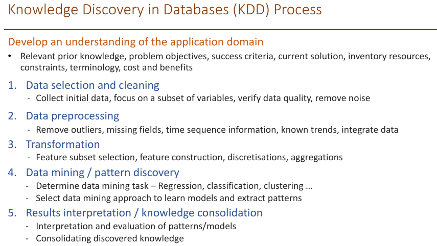
2. data

defination
- collection of data objects and their attributes
- attribute is a property or characteristic of an object
  - discrete/continuous
  - nominal: values are distinct symbols
    - ID, eye color, zip codes
  - ordinal: impose order on values but no distance between values defined
    - military rank, exam grade, rating
  - interval: has a fixed size of interval between data points
    - year, temperature
  - ratio: same as interval,0 means does not exist
    - weight, age
data quality
- noise
- outliers
- missing values
- duplicate

3. linear regression

$R^2$ higer better
- means that most of variation in yi data can be attributed to their corresponding x values
- higher if the data points aligned along a line
- should not inlude x unrelated to y in the model, just make R better
- adjusted R, use a penalty on the number of perdictors
underfitting and overfitting
- model complexity: the number of independent parameters to be fit, degree of freedom
- complex: more sensitive to data, more likely to overfit
- simple: under fit, rigid
- find the model balance bias-variance
- regularisation- ridge regression
  - x change slightly, y change al lot , not stable, not smooth
  - to encourage the weights to be small, resulting in a smoother curve
  - Solution: add a regularisation term to encourage the weights to be small, thus resulting in a smoother curve
  - - lamda*sum(wi^2)

4.logistic regression

Lorgistic Regression
- Y is categorical, binary, instead of continuous
- p = w1x1+w2x2+…+wixi=wTx
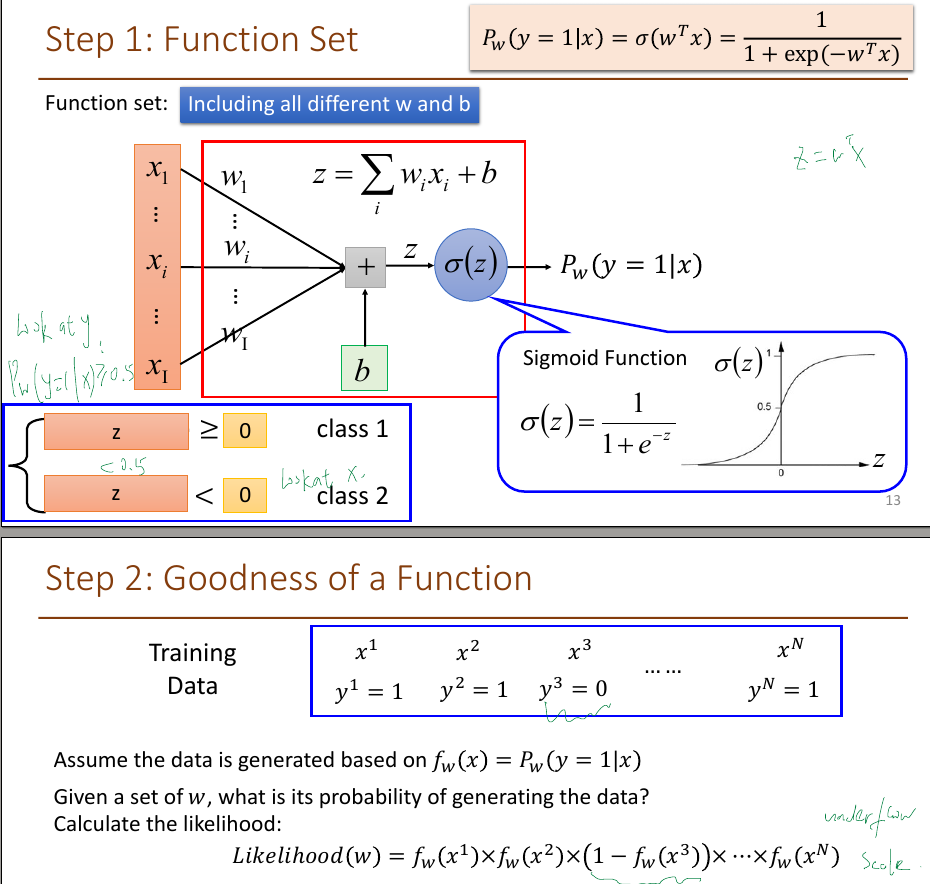
- sigmoid function
  - f(z), f = $\frac{1}{1+e^{-z}}$
  - use a non-linear function of the predictors to ensure p is within [0,1]
  - output can be interpreted as posterior label probability or confidence returned by classifier
    - p(y=1|x)+p(y=0|x)=1
    - p(y=1|x) = f(wTx)
    - p(y=0|x)= f(-wTx)
model parameter estimation
- step1, function set, including all different w and b. output between 0 and 1
- step2, goodness of a function, find w that minimises the cross-entropy between target class distribution(1 ,0 here, not a real number) and the predicted class distribution(probabilities)
- step3, find the best function
- why not squared error?
  - more severe plateaus with the squared error cost, too flat, the update is too small
  - cross-entropy cost works much better for classification problems
comparison
- yn, 1 for class1, 0 for class2; yn, a real number
- same update formula
multi class classification
- using the softmax instead of sigmoid
- the probablity sum = 1
- one hot output, 0 0 1
- still try to minimize the cross entropy
limitation
- feature transformation. new feature sapce
- deep learning: all the parameters of the logistic regressions are jointly learned

5.decision tree

Focus on class 1 and 2. In A ,3 class 1, 3 class 2

classification defination overall
- inexpensive to contrust
- fast at classifying unkonwn records
- easy to interpret for small-sized trees
- accuracy is comparable to others for simple datasets
pre-pruning: early stopping rule
- before it fully grown
- stop if same class/similiar/threshold
- stop if information gain improve
- stop if distributon of instances are independent of the available features
post pruning
- grow to its entirety
- trim nodes in a bottom-up fashion
  - if misclassification error decreases after trimming, replace by a node
  - use majority to replace

6. knn and nb

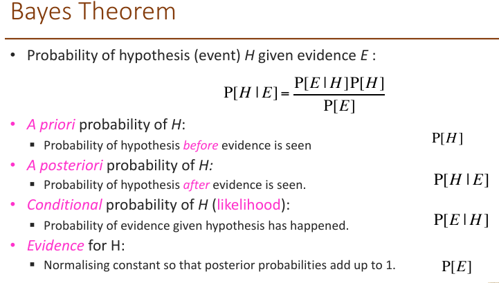
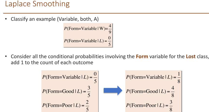
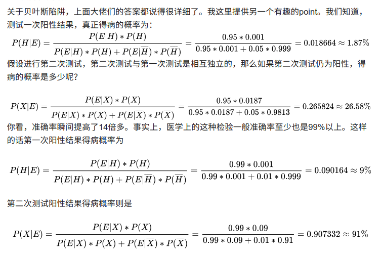
why nb still work?

classification doesn’t require accurate probability estimates as long as maximum probability is assigned to correct class

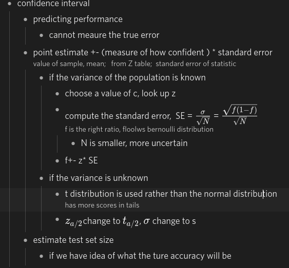
7. model evaluation

7.1 data split

large availalbe: holdout method, split training and test, build using training set and evaluate using test
parameter tuning
- test data must not be used for tuning any parameter
- proper procedure use valiedation data, to optimise/choose parameters
once evaluation complete, all data can be used to build
- the larger tarining, the better the classifier
- the larger test, the more accurate the error estimate
stratified sample: advanced version of balancing the data
- for small datasets usually
- make sure that each class is represented with approximately equal proportions in both subsets

7.1.2 k fold

avoids overlapping test sets, often subsets are stratified before
the error estimates on each subset are averaged
1. split into k subsets with equal size
1. each subset in turn is used for testing and the remainder for training

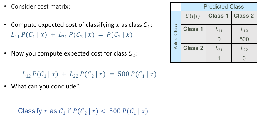
7.2 model evaluation metrics

binary classifiers generally have a postive and negative class, errors can only go the other class
- confusion matrix
  - precision=tp/tp+fp
  - recall = tp/tp+fn (ture positive rate TPR) tp and fn: gold stanard label, acutal positive
  - FPR false positive rate= fp/fp+tn
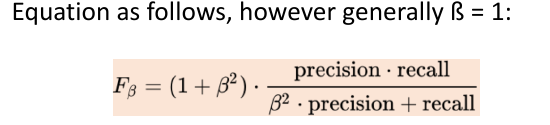
  - F = 2 precision*recall/(presion+recall)
multi-class may have differnet level of importance, error can go any others
- overall acuracy
  - 0.97 accuracy , misleading
- per-class precision/reacall
  - same as binary, also have per-class F1 score
- overall performance
  - macro-averaging-each
    - computer each, then avg, all classes contribute the same to final score
  - micro-averaging-all
    - compute overal, large classes contribute morel
multi-label instance can have multiple labels
- combinations of categories can have a new category
  - c1, c2, c3, c1c2, c2c3…
- two approaches to evaluate
  - hamming loss
    - just count wrong labels in the prediction matrix
    - 4*5 20 numbers, 4 wrong, 4/20
  - 0/1 loss
    - part incorrect is incorrect
    - 3/5
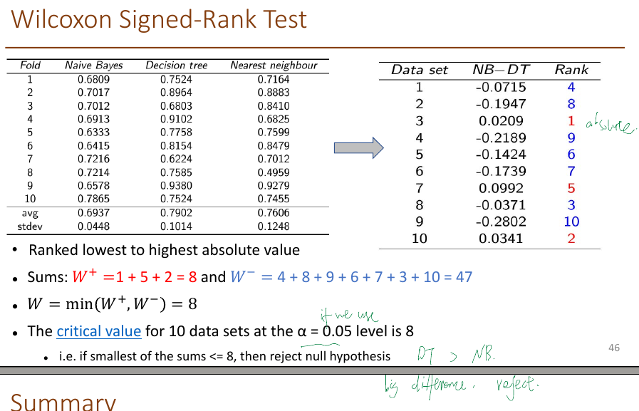
model comparison
- ROC Receiver operating characteristic
- TPR(recall) on y, against FPR on x
- change the thresholld , use classifier that produces posterior probability for each test instance P(+|A), count the number of TP FP TN FN at each threshold

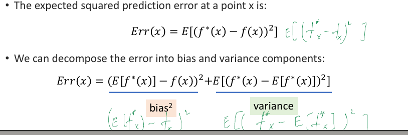
8. bias and variance

9. dimensionality reduction

principal component analysis PCA
- basic
  - some features may be correlated with each other, redundant
  - find a new set of features, linear combination of original
  - new features capture the maximum variance of data points
  - achieve the minimum reconstruction error
- PCA algorithm PCs are a series of linear least square fits to a sample, each orthogonal to all the previous PCs
- other
  - take enough many eigenvectors to cover 80-90 of variance
  - another point: minimising the error
  - weakness
    - assumption on linearity. non-linear methods such as kernel PCA
    - principal components are orthogonal, independent component analysis ICA
    - statistical importance of mean and variance, uses eignevector of the covariance matrix, does not count class label. no guarantee that the directions of max variance will contain good features
    - large variances have important dynamics, when data has high signal-to-noise ratio
neighbour embedding
- manifold learning(nonlinear dimensionality reduction)
- locally linear embedding LLE
  - find nearest neighbours, compute weights that best describing the point as a linear combination of neighbours
  - Use an eigenvector-based optimisation technique to find the low-dimensional embedding of points
- T distirbuted stochastic neighbor embedding t-SNE
  - basic
    - converts affinities of data points to probabilities, represeted by t-distributions rather than Gaussian joint probabilities, in order to allow dissimilar objects to be modeled far aprt in the map
    - sensitive to local structure which is highly preserved
    - compute similarity between all pairs of x and z, find a set of z making the two distributions as close as possible, z<x for dimension
  - disadvantage
    - computationally expensive, PCA is faster
    - stochastic, different seeds can yield different embeddings
    - global structure is not explicitly preserved. mitigated by initialising points with PCA

10. ensemble

10.1 framework of ensemble methods

train a set of classifiers from different training data(most adapted version, resampled for machine learning), combine the outcomes of different models (also two things in common with machine learning) average complex models to reduce variance
pros
- performace better than individual
- resilience to noise
cons
- time consuming
- hard to explain models

10.2 bagging

bagging: bootstrap aggregating
A simple but highly effective ensemble method that creates diverse models on different random samples of the original data set.
These samples are taken uniformly with replacement and are known as bootstrap samples.
combination: creating tree from random sub-sample of the features

10.2.1 random foreset

ensemble of decision trees, have high variance depending on the training data
- decision tree
  - easy to achieve null error on training data if has own leaf
- random forest bagging of decision tree
  - Train multiple trees on randomly sampled training data
  - randomly restrict the features used in each split – feature bagging
- out of bag OOB validation for bagging, good error estimation of testing set
  - mean prediction error on each training sample xi, using only the trees that did’t have xi in their bootstrap sample

10.3 boosting

boosting-adaboost consider the performance of previous models on the same data
- boosting D,T,A.
  - data set D. ensemble size T learning algorithm A
  - train an ensemble of binary classifiers from reweighted training sets
  - output: weighted ensemble of models
  - multiple weak linear classifiers combined to give a strong, non-linear classifier
- steps
  - 1. Train a weak model on some training data.
  - 1. Compute the error of the model on each training example.
  - 1. Give higher importance to examples on which the model made mistakes. weigh errors of the misclassified cases higher, correctly lower
  - 1. Re-train the model using “importance weighted” training examples. traning f2 on the new training set that fails f1, based on new weights u2. change the cost/objective function
  - 1. Go back to step 2.

10.4 bagging vs boosting

both reduce variance and overfitting
bagging can’t reduce bias, boosting can
- in boosting, training error steadily decreases
bagging performs better. if we don’t have a high bias and only want to reduce variance(if we are overfitting)
- bagging more computationally efficient, can train M models in parallel

11. Intro to DL

basics
- fully connect feedforward netwrok
- the unit of a neural network: activation function
  - combination function the unit combines its inputs into a single value
  - transfer funciton transform to produce the output
- softmax classifier
  - maxmise the probaility of the correct class, minimise the negative log probabilty of that class
- corss-entropy loss, find the parameters to minimise total loss

12. backpropagation and gradient descend

12.1 backpropagation

need to find the gradient of the error, w.r.t. the parameters of each layer,$\frac{dL(\theta)}{dw_k}$, to perform updates:
$w_k=w_k- \eta *$, $\frac{dL(\theta)}{dw_k}$ , $\eta$ is learning rate, wk is update weight
Forward pass: compute z and a for all layers
Backward pass: compute dz/dw and dl/dz for all layers

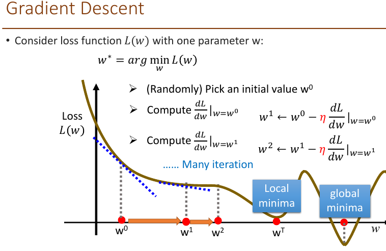
12.2 gradient descent

gradient descent: computes the gradient of the cost function w.r.t. the parameter for the entire training dataset, then perform one update
- slow, loss is the summation over all training examples
- $\theta^{t+1}=\theta^{t}-\eta^t*\nabla L(\theta^t)$
stochastic: performs a paramter update for each training example xn and label yn, make the training faster
- loss for only one example
- high variance, if 20 examples, 20 times faster
- $\theta^{t+1}=\theta^{t}-\eta^t*\nabla L^n(\theta^t)$
- L is different here, no sum
minibatch gradient descent
- between above two, updates for every mini batch of m training examples
- reduce the variance of the parameter update, lead to more stable convergence
- make use of matrix optimisations
adaptive learning rates
- reduce the learning rate by some factor every few epochs
- at first large, close to destination, reduce
Adagrad differnet learning rate for different parameters
- core
  - divide the learning rate of each parameter by the root mean square of its previous derivatives
  - provides a feature-specific adaptive learning rate by incorporating knowledge of the geometry of past observations
- smaller updates for parameters with frequently occurring features, larger for infrequent
- weakness stop learning
  - its accumulation of the squared gradients in the denominator
  - Since every added term is positive, the accumulated sum keeps growing duringtraining.
  - This in turn causes the learning rate to shrink and eventually become infinitesimally small, at which point the algorithm is no longer able to acquire additional knowledge.
RMSProp
- divides the learning rate by an exponentially decaying average of squared gradients
- high weight for current factor

13.CNN

overview
- neural networks that use convolution in place of general matrix multiplication in at least one layer
- why for image
  - 1.some partterns are much smaller than the whole image
    - a neuron does not have to see all, connecting to small region with less parameters
  - 2.the same patterns appear in different regions, could reuse
  - 3.subsampling the pixels will not change the object less parameters for the network to process the image
- Convolution(12)-maxpolling(3)-covolution-maxpooling-flatten-fully connected feedforward network
convolution layer
- those filter matrx are the network parameters to be learned
- each filter detects a small pattern
- output size
  - N is the row of orginal, K is the filter size, S is the stride size
  - used N=6, K=3, S =1
  - (N-K)/S + 1
- zero padding
  - output have the same size of input.
  - stride 1 ,filter k, padding with (k-1)/2
  - k=5, padding with 2, means 2 left, 2right
    - output size: (32+2*2-5)/1+1=32
    - number of parameters:
      - each filter:5*5+1=26 (+1bias)
      - 26*6 = 156
pooling layer
- max pooling: pick largest value from each filter
- the number of the channels is the number of filters
- smaller than original image

14.RNN

recurrent neural network good at dealing with sequence input and/or output
- process a sequence of vectors x by applying a recurrence formula at every time step
- ht = fw(ht-1, xt)
  - new state, some function with parameters w, old state, input vector at some time step
- the same function and the same set of parameters are used at every time step.
- unfortunately
  - not always easy to learn
  - The error surface is either very flat or very steep.
simple RNN
- the state consists of a single hidden vector h
- re use the same weight matrix at every time-step
- Elman and Jordan
  - Elman:a three-layer network with the addition of a set of “context units”
  - Jordan: the context units are fed from the output layer instead of the hidden layer.
- bidrectional RNN last word, first input
backpropagation through time
- Forward through entire sequence to compute loss, then backward through entire sequence to compute gradient
- Truncated backpropagation part , not whole
  - run forward and backward through chunks of the sequence instead of whole sequence
  - Carry hidden states forward in time forever, but only backpropagate for some smaller number of steps
Vanilla RNNs gradient flow suffer from gradient vanishing/explosion problem
- backpropagation from ht to hk multiplies by WhhT many times
- exploding gradients: WhhT large
  - gradient clipping, scale gradient if its norm is too big
- vanishing gradients: change RNN architecture:LSTM

15 word embedding

feature generation: bag of words Text document is represented by the words it contains (and their occurrences)
- dis: inefficient for large vocabularies
- does not capture semantics. each word is an unrealted token,
- ignore the word order
word weighting
- TFIDF(w) = tf * log(N/df(w))
- term frequency(occur in a document) and document(containing word) frequency
- N number of all documents
document representation as vectors- Vector space model Represent a document by a term vector
- Term: basic concept, e.g., word or phrase
- Each term defines one dimension – N terms defines a N-dimensional space
- Term weights – can be the raw term frequency or TFIDF
word embedding learning
- representing words
  - A word’s meaning is given by the words that frequently appear close-by
  - representing words by their context(within a fixed size window) words appear nearby
  - use the many contexts of w to build up a representation of w
- word embedding can also reduce dimensionality, capture semantics, big-of words can’t.
  - count-based methods word-word matrix, term-context matrix
    - Build a word co-occurrence matrix from textual data
      - two words are similar in meaning if their context vectors are similar
    - Weighting by TFIDF/PPMI or performing Singular Vector Decomposition (SVD) on the count
      - PMI(w1,w2) = log2 P(w1,w2) / Pw1*Pw2 do words 1 and 2 co-occur more than if they were independent?
      - tfidf and PPMI are sparse representations
      - alternatively, representing words using dense vectors which are short and dense
    - matrix
    - GloVe Encoding meaning in vector differences
      - insights: Ratios of co-occurrence probabilities can encode meaning components
      - shows the connection between the Count work and the Predict work
        an appropriate scaling and objective gives Count models the properties and performance of the Predict models
  - prediction-based methods
    - the probability for each word as the next word wi
    - word2vec
      - basic
        Instead of counting how often each word w occurs near “apricot”
        • Train a classifier on a binary prediction task: Is w likely to show up near “apricot”?
        • We don’t actually care about this task But we’ll take the learned classifier weights as the word embeddings
      - insights:
        a word w near apricot acts as gold correct answer to the question ' is w likely to show up near apricot'
        using running text as implicitly supervised training data
      - word2vec: skip gram task “skip-gram with negative sampling” (SGNS)
        1Treat the target word and a neighbouring context word as positive examples
        2.Randomly sample other words in the lexicon to get negative samples
        3.Use logistic regression to train a classifier to distinguish those two cases
        4.Use the weights as the embeddings
    - fasttext

16. VAE

Autoencoder Unsupervised approach for learning a lower-dimensional feature representation from unlabelled training data
- dimensionality recution here, want features to capture meaningful factors of variation in data
- how to train: Train such that features can be used to reconstruct original data
  - “Autoencoding” – encoding itself
- problem
  - The latent space where the encoded vectors lie may not be continuous, or allow easy interpolation
  - But when building a generative model, we don’t want to replicate the same image seen before. We want to generate variations on an input image from a continuous latent space.
- De-noising auto encoder, add noise
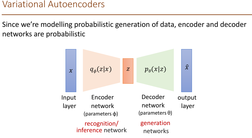
Variational Autoencoder (VAE) their latent spaces are, by design, continuous, allowing easy random sampling and interpolation.
- basic
  - The encoder of VAE outputs two vectors of: a vector of means, μ, and another vector of standard deviations, σ
    - Instead of an encoding vector as in standard autoencoder
  - We then sample from N(u,σ^2) to obtain the sampled encoding, which we pass onward to the decoder
  - The decoder is exposed to a range of variations of the encoding of the same input during training
    - The decoder not just decode single, specific encodings in the latent space (leaving the decodable latent space discontinuous), but ones that slightly vary too
- Intuition: x is an image, z is latent factors used to generate x such as attributes, orientation, etc.
- intractable problem
  - learn model parameters to maximise the likelihood of training data
  - data likelihood:
    - p(X) = $$\int p(z)p(x|z)$$
    - intractable to compute p(X|Z) for every z
    - Posterior density also intractable: P(Z|X)
  - inaddition to decoder network modeling P(X|Z), define additoinal encoder network q(Z|X) that approximates P(Z|X)
- evidence lower bound ELBO max it
- reparameterisation trick
  - Problem: cannot do backpropagation for a random sampling process
  - Solution: reparameterisation trick
    - • randomly sample ε from a unit Gaussian
    - •shift ε by the latent distribution’s mean μ and scale it by the variance σ

17. GAN

motivation
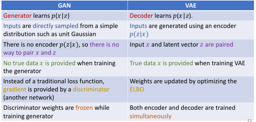
- VAEs define intractable density function with latent variable z, Cannot optimise directly, derive and optimise lower bound on likelihood instead
- give up on explicitly modeling density, and just want ability to sample?
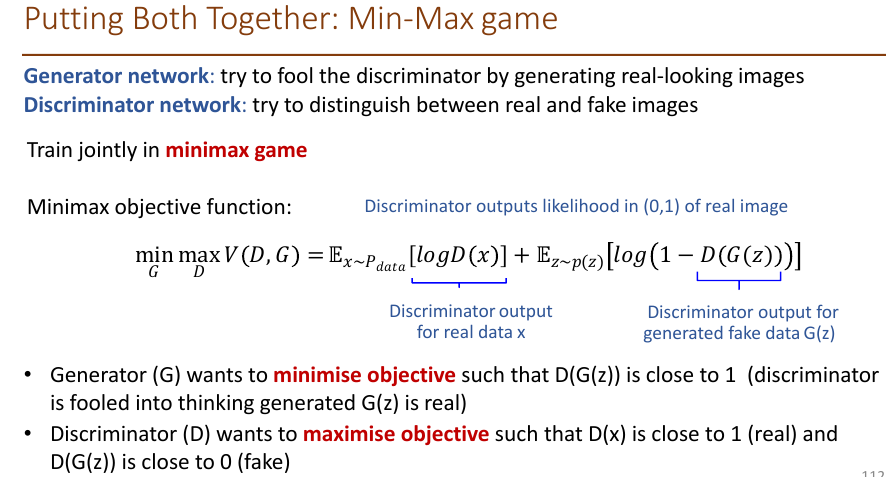
- GANs: learn to generate from training distribution through 2-player game
  - Generator network: try to fool the discriminator by generating real-looking images
  - Discriminator network: try to distinguish between real and fake images
basic idea of GAN
- Generator P(x) is a Neural Network
- The discriminator tries to learn P(y|x), where y is the label, 0 (generated) or 1(real), and x is the real or generated data.
- The discriminator essentially defines a new metric
- loss function- Minimax objective function
  - Generator (G) wants to minimise objective such that D(G(z)) is close to 1 (discriminator is fooled into thinking generated G(z) is real)
  - • Discriminator (D) wants to maximise objective such that D(x) is close to 1 (real) and D(G(z)) is close to 0 (fake)
- training
  - D repeat k times, G only once
  - stationery point
    - the generated data exactly matches the distribution of the real data
    - the discriminator is outputting a constant value for all inputs
comparion between GAN and VAE