High-performance computing module outline

March 10, 2019

warwick

For Warwick University module 402, high performance computation.

1.Fundamentals

1.1 the technologies needed to support HPC

computer architecture
- CPU, memory
- VLSI, transistors
- multicore, to ease the density(temperature etc.)
- GPU
networking
- bandwidth, latency
- communication protocols
- network topology
compilers
- identify inefficient implementations
- make use of the characteristics of the computer arcitecture
- choose a suitable compiler for a certain architecture
algorithms
- design
- parallel
- paradigm of parallel programming
workload and resource manager
- task scheduling and resource allocation
- metrcs

1.2 Evolution of HPC, difference

1960 scalar processor
- process one data item at a game
1970 vector processor (GPU is one)
- can process an array of data items in one go
- architecture: one master processor and many math coprocessors(ALU), not independent
- each time, the master processor can fetch one vector of data items and an operation, feed them to ALUs
- overhead:more complicated address,data fetching procedure
1980 MPP massively parallel processing
- up to thousands processors with its own independent memory
- processors can fench and run instrustions in parallel
- break down the instructions(workload) in parallel
- workload balance and processor communication(as little as possible)
- blue gene: a massive number of low performance processors
- not every processor has full function, e.g. IO
1990 cluster
- connecting each stand-alone computers with high speed network
- using commodity computer, good portability
1990 grid
- further evlotion of cluster
- integrate geographically distributed resources
2000 cloud
- commercialization of grid and cluster computing
- resources and services provided by the third party

1.3 Shared memory and distributed memory

shared memory(SMP)
- multiples CPUs, single memory
- all resources are equally available to each core
- do not scale well, requre critical section, cache is critical
shared memory(Non uniform memory access:NUMA)
- multiple CPUs
- each CPU has fast access to its local area of the memory, slower to other remoter(switch first, then router)
- scale better, hierarchical memory access
- complicated memory access patter
- global address space
distributed memory (MPP, cluster)
- each CPU has own independent memory
- interconnected through over-cable networks
- share data need an explicit communication, MPI e.g.
- larger latencies between processors
- better scalability

1.4 Instruction dependency

control dependency: if then
data dependency
- flow a=b+c, d=a+c
- output d=a+c, d=a+e
- anti a=b+c,b=2*e
- output and anti could be removed by rename

1.5 Parallel, distributed computing

parallel
- breaking the problem to be computed into parts that can run simultaneously
- eg: MPI perform matrix
- solve tightly problems
parts of work are computed in differernt places
- does not need simulaneous processing
- eg: workflow in a Grid
- loosely-coupled problems, not much communication

2.OpenMP

assist compilers to understand the serial program, automatically parallelize it
used in shared memory parallelism
an implementation of thread models

2.1 3 ypes of components

global data(heap, shared among threads)
code(executing)
stack(local private data, not shared)

2.2 differences between creating new processes and new threads

create process

use the fork function, all three segments and the program counter are duplicated

create thread

only the stack segment and program counter are duplicated
Light weight process”: multiple threads exist within the context of a single process, sharing the process’s code, global information, other resources
Used to split a program into separate tasks, one per thread, that can execute concurrently

2.3 what are OpenMP directives used to specify

sections of code that can run in parallel
critical sections
scope of variables (private of shared)

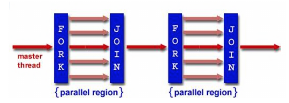
2.4 fork-join model

multiple threads are created using the parallel directive.

2.5 determine the number of threads generated in OpenMP

omp_set_num_threads() library function
OMP_NUM_THREADS environment variable
default, the number of CPUs on a node

2.6 scheduling iterations of loops to threads

Compiler directive specifies that loop can be done in parallel
Use thread scheduling to specify partition and allocation of iterations to threads
partiion the loop into blocks of iterations of size chunk

partition and allocation of loop
- # pragma omp parallel for schedule(static,4) before execution, the difference between dynamic
  - partiion the loop into blocks of iterations of size chunk
  - 1-4 first, 4-8 second thread
  - Before execution, deal out the blocks to each thread
- dynamic
  - put blocks into a queue
  - partiion the loop into blocks of iterations of size chunk
  - during execution, each thread grabs a block off the queue until all are done,
  - which thread runs which block of iterations depends on the execution pace
- schedule(runtime)
  - find schedule from an environment vaiable OMP_SCHEDULE
synchronisation
- critical construct one block per thread protected
- barrier one too fast, then wait

2.7 data scope attributes in OpenMP

data scope:define how variables should be viewed by threads
- shared(var)
  - states var is a global variable to be shared among threads
- private
  - creates a local copy for var for each thread
- reduction(operation: var)
  - a local copy of var made for each thread, updated by threads, same as private
  - at then end, local values are combined through the reduction operation

3.Programming models

3.1 what can compiler approach help in Parallel comuting?

automatically parallelize the sequential codes
very conservative
reimplementing the code in an more efficient way
remove the dependency if possible

3.2 data parallelism

3.2.1 data parallelism vs task parallelism
- Task parallelism: multiple processors run different operations
- Data parallelism: multiple processors run the same operation on different elements of a data structure
3.2.2 why data parallelism is higher level than message passing
- programmer does not need to specify data partition and thread communication sturctures
- this is done by the compiler, inferred from the program and underlying computer architecture
- not all algorithms can be speicfied in data parallel terms
- if the program has irregular communication patterns then this will be compiled less efficiently

3.3 how are the threads in OpenMP generated physically?

only the stack segment and the program counter are duplicated, global data and executing code are not duplicated
Thread creation and running in OpenMP is implemented by calling the multi-threading APIs in POSIX operating systems
For example, during the compilation, if OpenMP compiler realizes that the threads need to be generated, it inserts the instructions of invoking the relevant API provided by OS

3.3.1 multi-threading and multi-processing API in OS

OS supported multi-threading(kernel space thread)
system call for scheduling processes, user ask system to invoke

3.4 multiprocessing

3.4.1 key functions of creating processes in C
fork() is used to create a child process
3.4.2 how to make different processes to run different tasks
The child process is exactly the same as the parent except the returned value of fork()
Use parent and child to do different tasks, pid = 0 for child process
3.4.3 overhead of swithching processes
when to switch (time for scheduling)
- time slice runs out
- system call, user ask system to invoke
- trap, fault -> fault handler
overhead of switching is high, have to save and load much information
- three segments, heap, code ,stack
- open file descriptors
- signal handler table
- program counter

3.5 multithreading

3.5.1 key functions of creating threads in C
- pthread_create create new thread of execution that runs specified procedure with specified arguments
- pthread_join wait for the return from a specified thread
- mutex
  - pthread mutex lock()
  - critical section
  - pthread mutex unlock()
3.5.2 user space thread and kernel space threads
- scheduling user space thread
- user threads exist within a process, managed by process
- no time slice for each thread, unlike process switching
- when multiple threads are allocated to same cpu core, need to call thread switching explicityly so each has opportunity to run
- without switching, a thread may hog the CPU so as to starve other threads
- only stack need to be load/store information
kernel space thread(OS managed)
- same as process:
  - time slicing
  - system calls
  - traps
3.5.3 overhead of swithching threads
- user space: user space threads usually switch fast
- kernel space: the switching overhead stands between processes and user space threads

3.6 synchronization

two types: mutual exclusion and cooperation

3.6.1 techinques for synchronization

Mutex to address mutual exclusion
wait and notify to address cooperation

3.6.2 how synchronization is implemented in C

critical section:section of code that access the global shared data and therefore should be accessed by one thread at a time
Mutex, used to enforce mutual exclusion of threads in a critical section
two states: lock and unlock
- initially unlocked, entering then locks, blocks others
- pthread_mutex_lock(&lock), critical section, unlock

3.6.3 how synchronization is implemented in Java

java monitor
- automatically generated for a class or object by library
- the monitor can be associated with the methods/statements in the class called synchronized methods or steatements
- the synchronized codes are called the monitor region regreaded as the critical section, therefore should be run by one thread at a time

3.6.4 synchronized methods and statements

methods
- addc1 and addc2 methods are with monitor of classA, can’t run concureently, associated with the same monitor(class related)
statements
- synchronized statements must specify the object that provides the lock,
- synchronized(lock1){},synchronized(lock2){}
- can run concurrently,
- can imporve concurrency with fine-grained synchronization

3.6.5 the ways of creating new threads in Java

1. extend the Threads class or implement the Runnable interface
1. extend or implement the run method in the Threads class or in the Runnable interface, run specifies what thread should do
1. create a new instance of the class for each thread
1. invoke the start method in the instance, start initializes a new thread of control that executes the run method

3.6.6 differnece between synchronization in Java and C

java provides built in , part of the programming language, higher level, not explicitly
C: mutex

4.MPI

Message Passing is the most widely used parallel programming model
Message passing works by creating a number of processes, uniquely named, that interact by sending and receiving messages to and from one another (hence the message passing)
Message passing programs are based on standard sequential language programs (C/C++, Fortran), augmented with calls to library functions for sending and receiving messages

4.1 OpenMP vs MPI

• MPI is used on distributed-memory systems • OpenMP is used on shared-memory systems • Both are explicit parallelism • OpenMP is higher-level control

Compiler can automatically parallelise the codes when instructed • MPI is lower-level control
Data partition, allocation and process communication are conducted by programmers

4.2 why the parameters in MPI_send and recv?

(address, count, datatype)
- data may not occupy contiguous memory locations
- storing format for data may not be the same in platform
- can construct their own datatype, handle non-contiguous data
message tag: message matching. differentiate the message from the same process(sender)
communicator: consists of a group of processes and a communication context, bring efficiency.

4.3 collective operations

MPI_Reduce:performs op over the data in the sendbuf and put result in recvbuf in root process e.g.min max
- root:all , as to be recv
- other: no recvbuf, as to be sent, no op
MPI_Allreduce:put back to recvbuf in all processes
MPI_Barrier(comm):synchronize all processes, no processes return from function until all processes have called it
MPI_Bcast:send same data from one to all
- (buff,count,type) treated by root as data to be sent, other as to be received
MPI_Gather:gather data from all to one
- root: all parameters.
- other: no recvbuf, recvcount, recvtype
MPI_Scatter:scatter different data from one to all
- root: no recv
- other: no send

4.4 modularity: how to create new communications

extract process group from communicator
MPI_Comm_split(comm, colour, key, newcomm)

color: control of process assignment, processes with same colour are in same new communicator, myid%3

4.5 application buffer vs system buffer in MPI

application buffer
- data buffer in MPI send/recv functions
- may copy several times
sys buffer
- hidden from the programmer and managed by the MPI library
- limited and can be easy to exhaust

4.6 Blocking and non-blocking communication, communication test

blocking communications
- blocking send: MPI_Send
  - sender doesn’t return until the application buffer can be re-used, which often means data have been copied from application buffer to system biffer. doesn’t mean that data will be received
- blocking recv: MPI_Recv
  - receiver doesn’t return until the data have been ready to use by receiver, often means data have been copied from system buffer to application buffer
non-blocking send/recv
- the calling process returns immediately
- Just request the MPI library to perform the communication: no gaurantee when this will happen
- Unsafe to modify the application buffer until you can make sure the requested operation has been performed (MPI provides routines to test this)
- Can be used to overlap computation with communication and have possible performance gains
testing non-blocking communications
- completion tests come in two types
  - Wait type
    - MPI_Wait(request, status) the communication specified by the request handle
    - block until the communication has been completed
    - non-blocking communication immediately followed by a WAIT-type test = blocking communication
  - Test type
    - MPI_Test(request, flag, status)
    - return immediately with a True of False value
    - the process can perform some other tasks if the communication has not been completed. could overlap.
- All and any
  - all
    - MPI_Waitall(count, array_of_requests, array of statuses)
      - wait for all communications to complete
    - MPI_Testall (count, array_of_requests, flag, array_of_statuses)
      - test if all communications have completed
  - any
    - MPI_Waitany (count, array_of_requests, index, status)
      - Query a number of communications at a time to find out if any of them have completed
    - MPI_Testany (count, array_of_requests, index, flag, status)

4.7 communication mode

standard mode
- basic
  - MPI_Send is the standard mode, the msgs are handled in the standard way, copied to system buffer
  - have acceptable performance, may not give the best in certain situations
  - blocking standard send and non-blocking standard send(same as efficiency)
- 2 questions
  - what happens next after the data has been copied to system buffer?
    - sender send ‘ready to send’, waits for a ‘ready to recv’ msg from receiver, transfer after recv that msg
    - receiver, when the receive routine is called, the MPI system sends a ‘ready to receive’ msg to sender
  - what happens if msg to be sent is bigger than system buffer?
    - the send routine will block until
      - the receive routine starts receiving data and therefore empty the system buffer;
      - the rest of the message has been copied to the system buffer.
    - p0 send A to p1, recv B to p1; p1 send B to p0, recv A to p0. If size of A exceeds system buffer?
      - p1 send B can return, no dead lock. wait for empty the buffer and available
    - A and B both exceed the sys buffer?
      - none can empty sys buffer, can’t go to recv both. dead lock
synchronous mode
- blocking : MPI_Ssend
  - routine doesn’t return until 1. data copied to sys buffer 2. MPI has received ready to receive(standard only 1. here?)
  - may incur overhead if receive routine is posted later than send routine
- non-blocking: MPI_Issend
  - return immediately
  - communication is considered complete only after 1.the data has been copied to sys buffer and 2. MPI sys received ‘ready to receive’ msg
buffered mode
- sender uses explicitly defined buffer instead of sys buffer
- communication is considered complete when 1. data copied to defined buffer(same as standard?)
- blocking buffered send : MPI_Bsend
  - must attach buffer space using MPI_Buffer_attach/detach
  - the size should be no less than the value: MPI_Pack_size(20,type1,comm,&s1) size = s1 + s2 + 2*MPI_BSEND_OVERHEAD
ready mode
- sender will send the data straightway without waiting for the ‘ready to receive’ msg
- when coder make sure the receive routine will be called before the send routine
- blocking ready send: MPI_Rsend, sender return until the application buffer can be reused
- non-blocking ready send: MPI_Irsend

4.8 Datatype

4.8.1 functions to construct derived datatypes
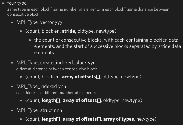
4.8.2 why can derived datatype improve the performance?
can handle non-contiguous data, with multiple datatype efficiently. otherwise:
- call send for each block, send multiple times
- cp to contiguous buffer space, then cp to sys, copy twice

5. performance and GPU

5.1 speedup, general trend of speedup

basic
- the imporvement or not brought about by parallelising an applicaiton code
- If n processors are used, S(n)=t1/tn
- maximum speedup for a parallel algorithm with n processors is n
- linear speedup is regarded as optimal
trend
- speedup increases as the number of PE increases
- the gap with maximum speed also increases
- after reaches maximum, futher adding processor elements PEs is no benefit and may harm performance
how to get a good S(n)
- algorithm design minimal sequential component and good percentage of inherent parallelism
- workload management balancing workload among processors
- get a high ratio of computation to communication when partition data effective work to overhead
  - reducing the impact of communication
    - minimize the amount of communication, with a good data locality
    - overlap communications with computation where possible
    - sending a few large messages
    - hardware, fast communications

5.2 parallel efficiency, isoefficiency

E(n) = S(n)/n, often S(n)« n speedup divdied by max
- same as the factors affecting speedup. typically greater n, low efficiency
ISO-efficiency
S(P)=T1/Tp, E = S(P)/P, e.g. when N=P, E remains constant as P changes
how the amount of computation performed N must scale with processor number P to keep parallel efficiency E constant
- the funciton of problem size N over P is called an algorithm’s iso-efficiency function
  - An algorithm with an iso-efficiency function of O(P) is highly scalable
    - Increase p by three times, only need to increase N by three times to maintain efficiency
  - An algorithm with a quadratic or exponential iso-efficiency function is less scalable
    - increase p by five times, need to increase N by 25 times and 32 times, respectively
- work out
  - find out how to make constant, N=O(P)

5.3 four approaches to modelling application performance

Speedup : this algorithm achieved a speedup of S on p processors with problem size N
- partitions the whole/expensive parts, introduce variable/fixed overhead
Amdahl’s law show the limitation of parallelising codes
- not amenable to parallelisation, serial fraction be f
  - Tn=$\frac{(1-f)T_1}{n} + fT_1$
  - S = T1/Tn = $\frac{n}{(1-f)+nf}$ <= 1/f
- can only tell the upper bound, cannot tell if exist greater parallelism
Asymptotic analysis
- the algorithm takes the time of O(nlog 2n) on n processors
- disadvantage:
  - ignore the low-order term( may counts when n is small)
  - only tell the order, not acutal time
modelling execution time
- performance model for the program
- an example - atmosphere model
  - discretize the space, use centre point to represent the whole cell
  - calculate the solution at these discrete points
- communication pattern

5.4 surface-to-volume ratio, usage of the ratio

The lower surface-to-volume ratio, the better: • Surface = communication • Volume = computation • means lower proportion of communication time in the whole execution time

1-D along y decomposition
- modelling computation time
  - each task is responsible for a subgrid of size N*(N/P)*Z
  - Tcomp = tc * N*(N/P)*Z, for each subgrid, tc is the avg time of calculating a single grid point
- modelling the time of sending one msg
  - Tmsg = ts + tw*L the time spent in sending one message
  - ts is the message startup time(overhead), tw is the transfer time per byte, L is the size of the message
- modelling communication time
  - Tcomm = 2(ts+tw*2NZ) Communication time for calculating a subgrid
  - Tp = Tcomp + Tcomm
- speedup S(P)=T1/Tp , T1=tcNN*P
- parallel efficiency E= (T1/Tp)/P
- ISO-efficiency, look at E, when N=P, approximately constant as P changes
2-D
- Tcomp = tc * N * (N/P) *Z same as 1D
- Tcomm = 4 (ts + tw*2 (N/$$\sqrt{P}$$)*Z)
- IOS-efficiency, when N = $$\sqrt{P}$$
- 2d bettter, drop slower with problem scale (only need increases 3 times when process increase 9 times) to keep the same efficiency

5.5 Design philsophy of CPU and GPU

how CPU interacts with GPU cards?

CPU could put some parts code which need to be computed by GPU according to instructions. Usually those pats are computation intensive.

CPU latency-oriended design
- optimize the performance of sequential code
- complicated control unit
- has large on-chip cache to reduce data access latencies
- powerful ALU arithmetic logic unit(each ALU area is big)
- at the cost of increased use of chip area and power

GPU thoughput-oriented desgin
- need to perform a massive number of floating-point calculations per video frame
- Motivate GPU vendors to maximize the chip area dedicated to floating point calculations
- each calculation is simple: therefore simple control logic and simgle ALUs
- calculation is more important than cache, therefore small cache, allowing memory access to have long latency
- a large number of simple ALUs on a chip to increase the total throughput
  - run with a large number of parallel threads, some waiting, can find other threads to run

5.6 execution of a CUDA program

_ _ global _ _ keyword
copy and input data and results between cpu memory and gpu memory
generate multiple threads according to execution configuration
different threads run different data items

5.6.1 3 steps

memory management in GPU: part 1 and 3
- cudaMalloc(void** devPtr, size_t size) allocate the device memory in GPU
  - devPtr: a pointer to the address of the allocated memory
  - size: size of allocated memory
- cudaMemcpy(dst, src, count, kind) memory data transfer
  - 1.destination location of the data to be copied
  - 2.source location of the data
  - 3.size of the data
  - 4.The types of memory copying: host to host, host to device, device to device, device to host
launch and run the kernel code: part2
- 1.Execution model of the kernel function
  - starts with CPU execution
  - when a kernel function is called, it executed by a large number of threads on GPU
    - all the threads are collectively called a grid
  - when all threads of a kernel complete their execution, the corresponding grid terminates
  - the execution continues on the CPU until another kernel is called
- 2.Thread structure
  - basic
    - when a host code launches a kernel, CUDA generates a grid of thread blocks
    - each block contains the same number of threads(up to 1024)
    - each thread in a grid runs the same kernel function
  - thread organization
    - two-level architecture: threads are organized into a grid of blocks
      - a grid has 3*2 blocks
      - a block has 4*3 threads
    - the grid and blocks can be multi-dimensional, their values are pre-initialized by the CUDA runtime library when invoking the kernel function, can be accessed in the kernel function
      - gridDim(x,y,z) 320
      - blockDim(x,y,z) 430
      - blockIdx(x,y,z)
        the coordinate ID of the block in the grid, obtain which block is in
        All the threads in a block share the same blockIdx value
      - threadIdx(x,y,z)
        the local coordinate ID of a thread in a block, to obtain its local position in the block
- 3.Execution configuration
  - specified when invoking a kernel function
  - set two parameters between «< and »> before the function parameters, gird and block dimension
  - stored in gridDim and blockDim
- 4.Workload distribution
  - differnet threads for differnet data, need to match threads(threadidx) to data items
    - Griddim(xyz)=(N,1,1), blockDim(xyz)=(256,1,1), N blocks, each with 256 threads
    - blockidx(x,0,0),threadidx(x,0,0), compute Cd=Ad+Bd
    - i = blockIdx.x * blockDim.x + threadidx.x
    - C[i] = A[i] +B[i]
  - only first n threads perform the addition
    - not all vector lengths can be expressed as multiple of the block size
    - allows the kernel to process vectors of any lengths
    - use if (i<n)
  - all threads in a grid run the same kernel function, use their coordinates to
    - distinguish themselves from each other
    - identify the appropriate part of the data to process

6.cluster

6.1 3 reasons why cluster regain in popularity

very high performance Microprocessors
High speed networking, communication
Standard tools for parallel/ distributed programming

6.2 what is the single system image: middleware

presents a collection of resources as a single powerful resource.
Simplified system management
Use system resources transparently
- Users need not be aware of the detailed resource information and underlying system architecture to use these machines effectively
Transparent load balancing and process migration across nodes.
Improved reliability and availability
Improved system-oriented performance
- • Global view of middleware vs. local view of a user

6.3 activities performed by a typical workload manager in clusters

queueing
- job submission two parts:
  - job description e.g. job name
  - describe the resource requirements eg amount of memory
- once submitted, jobs are held in the queue until the job is at the head of queue and the matching resources are available
scheduling
- Determining at what time a job should be put into execution on which resources
- There are a variety of metrics to measure scheduling performance
  - System-oriented metrics (e.g. throughput, utilisation, average response time of all jobs)
  - user-oriented metrics (e.g. response time of a job submitted by a user)
  - They can contradicts each other and balance needs to be made
monitoring
- Providing information to administrators, users and the Cluster manager on the status of jobs and resources
- The method of collecting the info may differ between different cluster manager, but the general purpose is the same
resource management
- handlinng the details of
  - Starting the job execution on the resources
  - Stopping a job
    - scancel 271276
  - Cleaning up the temporary files generated by the jobs
    - after the jobs are completed or aborted
  - Removing or adding resources
- For the batch system, the jobs are put into execution in such a way that the users don’t have to be present during execution
- For interactive systems, the users have to be present to supply information during the execution.
accounting
- for which users are using what resources for how long
- Collecting resource usage data (e.g. job owner resources requested by the job, resource consumption by the job)
- Accounting data can be used for:
  - Producing system usage and user usage reports
  - Tuning the scheduling policy
  - Anticipating future resource requirements by users
  - Calculating future resource allocations
  - Determining the area of improvement within the cluster

6.4 the two primary parts that a job submission script includes

job description e.g. job name
describe the resource requirements eg amount of memory
once submitted, jobs are held in the queue until the job is at the head of queue and the matching resources are available

6.5 what’s backfilling scheduling policy and its pros and cons?: fill the resource hole

the FIFO brings idle time, can be big
allows a job to start if it does not delay the execution of the first job in the queue.
utilisation is imporved
disadvantages
- information about the job execution time is required.
- User estimation are usually inaccurate.
- It is a policy decision to decide what to do if a job overruns;
- The default decsions is to terminate the job if it overruns
- Otherwise some users may deliberately underestimate the job length to get an earlier job start time.

6.6 Top500 list and the parameters(features)

ranked in terms of Flops: FLoating point Operations Per Sec
obtained by Linpack benchmark(scientific applications)
a measure of the capability of a computer in processing real numbers, represent parallel computers
why FLOP important?

It represent parallel computers, do not consider storage or IO issues. A real number is stored with the floating point format, which using a fiexed length space to store a wide overall range of values. Many scientific applications solve linear equations. The High Performance LINPACK (HPL) benchmark produces a FLOPS result. It solves a dense system of linear equations

features of scientific applications
- Calculating real numbers
- Data to be processed are often stored using matrix data structure (Linpack benchmark)
- High data locality (spatial locality and temporal locality)
- Cache is critical in performance: fetch the neighbouring data also. so next time . from cache

6.7 Graph 500, different features between scientific applications and graphbased applications

Use the metric to measure how fast a computer can traverse the edges of a graph, Gigasteps
features of graph based applications
- Have to store and access a large amount of data (intensive memory access)
- Need to establish the connections among data points
- The data are best stored using graph data structure
- Data locality is low
- Cache now has limited positive impact on performance
- A computer with a high FLOPS performance may not perform well with these graph-based applications

6.8 Gigasteps: another performance metric to measure and rank the supercomputers

Means “billions of traversed edges per second”
A node in the graph represents a data point
An edge is a connection between two data points.
Represent how fast a computer system accesses its global memory
Use the breadth-first search as the benchmark

7. cluster networking and IO

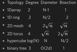
7.1 metrics used to measure the performance of switched networks

Scalability : the function of switch over nodes.
Degree: number of links to / from a node ,measure aggregate bandwidth
Diameter: the shortest path between the furthest nodes.measure latency
Bisection width: the minimum number of links that must be cut in order to divide the topology into two independent networks of the same size (+/- one node).
- measure of bottleneck bandwidth - if higher, the network will perform better under heavy load.
Communication time = time spent at the sender (latency at the sender) + datasize/bandwidth + switching time (latency at the switch) + time spent at the receiver (latency at the receiver)

7.2 given an network topology, calculate the quantities of the metrics

7.3 two switching techinques and their performance models

store and forward
- Each switch receives an entire packet before it forwards it onto the next switch - useful in a non- dedicated environment (I.e. a LAN).
- Since buffer size is limited, packets will be dropped under heavy load.
- impose a larger in-switch latency.
- Can detect errors in the packets
worm hole routing(cut though)
- Packet is divided into small “flits” (flow control digits).
- Switch examines the first flit (header) which contains the destination address, sets up a circuit and forwards the flit immediately.
- Subsequent flits of the message are forwarded as they arrive (near wire speed, i.e. at a speed close to direct connection).
- Reduces latency and buffer overhead.
- Less error detection
performance model for store and forward
- - Startup time Ts: the time required to handle a msg at the sending/receiving nodes:
- - Per-hop time Th: the in-switch latency.
- - Per-word transfer time Tw: if the link bandwidth is r, then Tw =1/r
- - Construct the performance model for the communication time of sending a message of size L through D links
- e.g.: Ts+(Th+Tw*L)*D , D=4 here
performance model for cutting through different filts in parallel
- Each message is broken into fixed units called flow control digits(flits).
- Flits contain no routing information.
- They follow the same path established by a header.
- Construct the performance model for the communication of sending a message of size L through D links under this switching technique
- e.g.: Ts+(Th+Tw*f)D+ Tw(L-f) secondpart: 1 so far ; third part: 2 3 4
  - 4 filts, f is size of filt1, L-f: other filts, no more Th here
  - the rest of flits are sent in parallel through links under cut-through switching

7.4 Granularity of parallelism

Defined as the size of the computations that are being performed in parallel

7.4.1 Four types of parallelism (in order of granularity size)

Instruction-level parallelism (e.g. pipeline)
- allow overlapping execution of multiple instructions
- factors that limit: can’t divide instructions infinitely
- need more function units, cannot put more transistor to cpu chip
Thread-level parallelism (e.g. run a OpenMP or GPU program)
Process-level parallelism (e.g. run an MPI job in a cluster)
Job-level parallelism (e.g. run a batch of independent jobs in a cluster)

7.5 three version of parallel IO, pros and cons

version1.0
- Assume 4 processes compute the elements in a matrix in parallel , All processes send data to process 0, which then writes to file
- bad
  - 1. Single node bottleneck
  - 1. Single point of failure
  - 1. Poor performance
  - 1. Poor scalability
- good
  - 1. The IO system only needs to deal with I/O from one process
  - 1. Do not need specialized I/O library
  - 1. If you are converting from sequential code then this parallel version (of program) is easy to implement
  - 1. Results in a single file which is easy to manage
version2.0
- Each process writes to a separate file, all prcesses can write in one phases
- good
  - now doing things in parallel
  - high performance
- bad
  - 1. We now have lots of small files to manage
  - 1. How do we read the data back when # procs changes?
  - 1. Does not interoperate well with other applications
version3.0- now version
- Multiple processes of parallel program access (read/write) data from a common file at the same time parallel I/O is now integral part of MPI-2
- all processes can write in one phase, to differernt parts of one common file
- good
  - Simultaneous I/O from any number of processes
  - Excellent performance and scalability
  - Results in a single file which is easy to manage and interoperates well with other applications
  - Maps well onto collective operations
- bad
  - Requires more complex I/O library support
  - Traditionally, when one process is accessing a file, it blocks the file and another process cannot access it.
  - Needs the support of simultaneous access by multiple processes

7.6 IO performance optimisation techniques

Data sieving
- combine lots of small accesses into a single larger one
- reducing the number of operations, more complicated
- read all, modify some, write back
- requires locking in the file system,can result in false sharing
collective IO
- problems with independent , noncontiguous access
- Collective I/O is coordinated access to storage by a group of processes
- must be called by all processes participating in I/O
- Allows I/O layers to know more as a whole about the data to be accessed
- First phase reads the entire block
- Second ‘phase’ moves data to final destinations

7.7 solution for disk failure

full redundancy: replication(mirroring)
partial redundancy: parity information XOR
- if any data is lost, we can recover the data from parity and the remaining data
- only one of the N+1 drives contains redundancy information
- parity information has to be computed every time the data is updated