For Warwick University module 918, natural language processing.
Question 1: Regular expressions, linguistic preprocessing, minimum edit distance algorithm.
1 regular expression
remember use \.
false positive type1: have output, shouldn’t. precision = tp/(tp+fp)
false negatives(type 2): haven’t output, but should minimise, increase recall recall = tp/(tp+fn)
F1= 2 precision* recall/(precision+recall)
2 text preprocessing
vocabulary size: the number of different types of tokens in the text.
All need 3 steps
- tokenizing/segmentting words in running text
- normalizing word formats
- segmenting sentences in running text
Issues of tokenisation
- What counts as a word is usually application specific. keep special characters (hashtags, URLs, email addresses) as words, in others we don’t.
- Commas and points in numbers can be confusing
- How to tokenise clitic contractions (i.e. I’m -> I am)
- How to deal with multi-word expressions (e.g. New York, San Francisco)
basic concept
| tokenisation | segmenting running text into words |
|---|---|
| normalisation | putting words/tokens in a standard format |
| Lemmatisation | reducing inflections or variants forms of words to their base form. Need to find dictionary headword form. |
| Stemming | finding the stem by stripping off suffixes, usually using regular expressions. |
Maximum Matching (also called Greedy) for Chinese:
- Start a pointer at the beginning of the string.
- Find the longest word in dictionary that matches the string starting at pointer.
- Move the pointer over the word in string.
- Go to 2
minimum edit distance
- minimum number of editing operations (operations like insertion, deletion, substitution) needed to transform one string into another.
- To find potential spelling correction
- to compute minimum cost alignment between two strings etc.
Question 2: N-grams, Language models, smoothing.
3 language models
ngrams
- A language model where we approximate each component in the product from the N-1 previous words
- N-gram can denote the above language model or the sequence of N words.
- unigrams, bigrams, trigrams and so on. may more detailed and sparse for longer n-grams.
Markov
- we can approximate the computation of such probability by only looking at the preceding item (or k preceding items) in the sequence, instead of looking at the whole sequence
- the longer the length, the more details, the more sparse
- P (wj |w1 …wj-1 ) = P (wj |wj - 1 )
- P(you, found) = P(found | you) = count(you found) / count(you) = 2/3
extrinsic and intrinsic
| Extrinsic | test externally on another task, accuracy using LM1 and 2, ideal but take very long to run |
|---|---|
| Intrinsic | evaluate the models directly. Consists in computing perplexity. |
perplexity:
- inverse to probability, lower is better.
- how difficult is it to predict the next word?
- the one that gives higher probability to the actual next word.
- Only valid if tested in similarly looking data.
4 advanced LM : smooth
| Smooth | Smoothing is the process of transferring a small amount of probability mass from observed n-grams to n-grams with 0 frequency. By using smoothing we allow our n-gram language models to generalise to unseen n-grams. |
|---|---|
| Laplace smoothing. | In order to fix the zero problem when training models, Pretend we have seen each word one more time than we actually did. In domains where the number of zeros isn’t so huge, not for N grams |
| Interpolation and backoff. | Different words may need different context size captured |
| Good Turing Smoothing. | se the count of things we’ve seen once to estimate counts of unseen things |
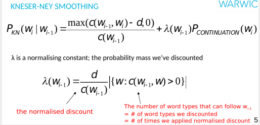
| Kneser-Ney Smoothing. | How likely is w to appear as a novel continuation.P(continuation) is the word types before w, divided by the number of differnet words that precede any word. lamda, there’s the word type after w(i-1). |
Question 3: Text/sequential classification, sentiment analysis, evaluation.
7 Text Classification, Evaluation and Error Analysis
- overfit : Overly adjusting our classifier and features to a specific training set and thus a particular test set similar to training data, and it will not generalise to new, unseen test sets.
- corss-validation:
- semi-supervised different : Semi-supervised classification also makes use of unlabelled data for training. A supervised classifier relies only on labelled data.
how to assess which features are good
- Incremental testing: keep adding features, see if adding improves performance
- Leave-one-out testing: test all features, and combinations of all features except one. when leaving feature i out performs better than all features, remove feature I
- Error analysis: look at classifier’s errors, what features can we use to improve?Look at confusion matrix, common features of errors, and potential imbalance in predictions
two different settings to develop multiclass classifiers?
- Multinomial:
- is generally faster, a single classifier.
- classes are mutually exclusive, no overlap.
- one vs all ( multi-label)
- Multilabel classification, K classes into K binary tasks, document can fall in 1+ categories
Macro and Micro-average
- Macroaveraging
- Compute performance for each class, then average them.
- All classes contribute the same
- Microaveraging:
- overall performance without computing per-class performances.
- Large classes contribute more
3 ways of dealing with imbalanced data in text classification, error analysis
- Undersample popular class by removing instances to balance it with the rest.
- Oversample the other classes to balance them.
- Create synthetic data for the classes with few training instances.
- Cost sensitive learning by assigning prediction probabilities to each class.
8 Sequence classification and POS
HMM Hidden Markov Models
- markov chain
- Set of nodes connected with probabilities, where weights on all edges leaving a node sum to 1.
- states, transition probability matrix, start and end state
- transition probability: tag followed tag
- HMM: + observations, observation likelihoods(emission probabilities)
- emission: tag to a particular word
- assumption
- dependence only on the previous state
- must be a dependency between sequence items
- Limitations of HMM:
- Models dependencies between each state and only its corresponding observation.
- Learns joint distribution of states and observations P(Y, X), but not the conditional probability P(Y|X).
MEMM Maximum Entropy Markov Models
Models dependencies between each state and the full observation sequence. Learning objective function consistent with predictive function: P(Y|X).
CRF Conditional Random Fields
Global normaliser Z(x) overcomes label bias issue of MEMM. Models the dependency between each state and the entire observation sequence (like MEMM).
comparision, overcome label bias
HMM have the limitation imposed by the Markov assumption, i.e. they only rely on the previous element in a sequence. MEMM suffer from a label bias, as it relies on global sequence probabilities as opposed to local probabilities. CRF overcomes these two limitations by relies on the entire sequence and by using a normaliser Z(x) to avoid the label bias.
Question 4: Parsing, information extraction, POS tagging, NER.
9 grammars and parsing
Parsing
- Parsing: process of recognising a sentence and assigning syntactic structure to it.
- Syntactic structure includes:
- Constituents: how words group together to behave as single units.
- NP PP VP
- Grammatical relations, dependencies, subcategorisation: how words and constituents relate to each other.
- Constituents: how words group together to behave as single units.
CFG context free grammers
- widely used mathematical system for model constituent structure
- three compontents
- terminals
- non-terminals
- rules: To produce grammatical sentence, consist of a single non-terminal on the left and any number of terminals or non-terminals on the right.
lexicalised PCFG
- considering the probabilities of words occurring in different constituents
- can deal with disambiguation better
CFG, PCFG and lexicalised PCFG
CFGs don’t have probabilities. PCFG s are more sophisticated than CFGs as they do include the probabilities associated with each rule and terminal. Lexicalised PCFGs are an improved alternative of PCFGs, to mitigate the lack of consideration of context. Besides probabilities of rules and terminals, lexicalised PCFGs also incorporate words within those rules. For instance, in the case of the sentence: “ I had pizza with friends”, the PCFG may find it equally likely to choose the rule NP -> NP PP and VP -> V PP but if words are added to the rules (i.e. NP/pizza -> NP/ pizza PP/with friends vs VP/ate -> V/ate PP/with friends) the VP rule would be much more likely.
CKY: bottom up, from sentence to tree
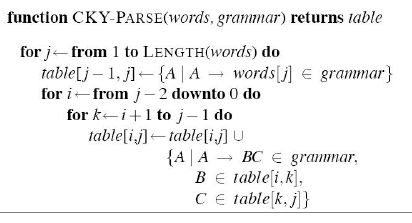
It is a dynamic programming algorithm used for parsing constituent trees. It starts by creating an empty tree with no labels. This tree contains all possible branches. It starts from the bottom elements, iteratively deciding the labels for the elements in the upper levels of the tree, by finding all possible combinations of terminal and non-terminal nodes encountered that match the right hand side of rules.
MaltParser algorithm for? 4 types opersations?
for dependency tree parsing. The four possible operations are left-arc, right-arc, reduce and shift.
dependency grammars
- Dependency syntax postulates that syntactic structure consists of lexical items linked by binary asymmetric relations (“arrows”) called dependencies.
- Graph Algorithms:
- Consider all word pairs.
- Create a Maximum Spanning Tree for a sentence.
- Transition-based Approaches:
- Shift-Reduce Parser: MaltParser.
- Similar to how we parse a program
- Graph Algorithms:
10 word senses and similarity
sense
Homonymy: same word can have different, unrelated meanings bank Polysemy: same word, related meanings: often systematic Synonyms: words with same meaning in some or all contexts Antonyms: Senses that are opposites with respect to one feature of meaning Hyponymy:One sense is a hyponym of another if the first sense is more specific, denoting a subclass of the other: apple of fruit hypernym: fruit is hypernym of apple
What are hyponyms and hypernyms, and what is the best resource we can use to identify them?
One sense is a hyponym of another if the first sense is more specific, denoting a subclass of the other: (1) car is a hyponym of vehicle, (2) apple is a hyponym of fruit. Conversely hypernym: (1) vehicle is a hypernym of car, (2) fruit is a hypernym of apple. The best resource for dealing with hyponyms and hypernyms are thesauri. They can be found in taxonomies and lexical databases such as WordNet.
thesaurus methods
- Thesaurus (plural thesauri) is a reference work that lists words grouped together according to similarity of meaning.
- path-based similarity: Two senses are similar if there is a short path between them in the thesaurus hierarchy
- Thesaurus-based similarity algorithms:
- Dekang lin similarity function
PMI
log P(x,y)/(pxpy)
11 information extraction and named entity recoginition
NER
Find each mention of a named entity in the text and label its type. What constitutes a named entity type is application specific; these commonly include people, places, and organizations but also more specific entities such as namesof genes and proteins. Statistical sequence models are the norm in academic research. Commercial NER are hybrids of rules & machine learning.
Question 5: Information retrieval, QA, text summarisation.
12 introduction to IR
query processing
- use skip pointers:skip all values smaller than 35 in p1., since p2 started with 35
- Longer n-gram indices are not feasible
- Bigrams could be used when we don’t need longer search queries, but it’s generally not enough.
- Use of bigrams to look for longer n-grams can lead to false positives (as with the “University of AND of Warwick” example)
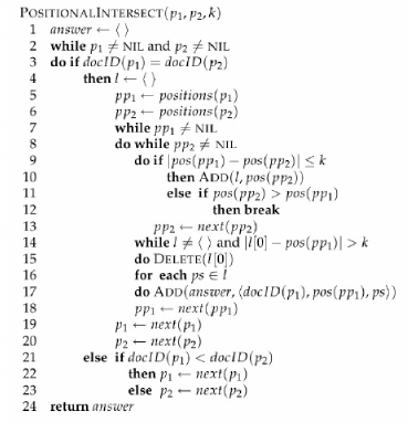
positional indices
- In the postings, store for each term the position(s) in which tokens of it appear:
- Get inverted index entries for each distinct term: to, be, or, not.
- Look for occurrences where the positions match the sequence of our query
- main dis:use more space than binary index
- main adv:flexibility for searching
13 ranking in IR
jaccard coefficient, TFIDF
- jaccard A^B/AUB
- TFIDF
- rare and frequent in a document
- weight of a term is the product of its tf and idf weights
- (1+logtf(t,d))*log(N/dft)
- term frequency:sum(1+logtf)
- inverse document frequency:log(N/df)
- dft is the number of documents that contain t.
- N = number of documents in collection.
SMART
Many search engines use different weightings for queries vs documents. The SMART notation denotes the combination in use in an engine, with the notation ddd.qqq for document (d) and query (q). There is a notation with different options for each of the 3 characters on each side. A very standard weighting scheme is: lnc.ltc:
- Doc: logarithmic tf (l), no idf (n) and cosine normalisation (c).
- Query: logarithmic tf (l), idf (t), cosine normalisation (c).
14 efficiency and evaluation of IR
PageRank
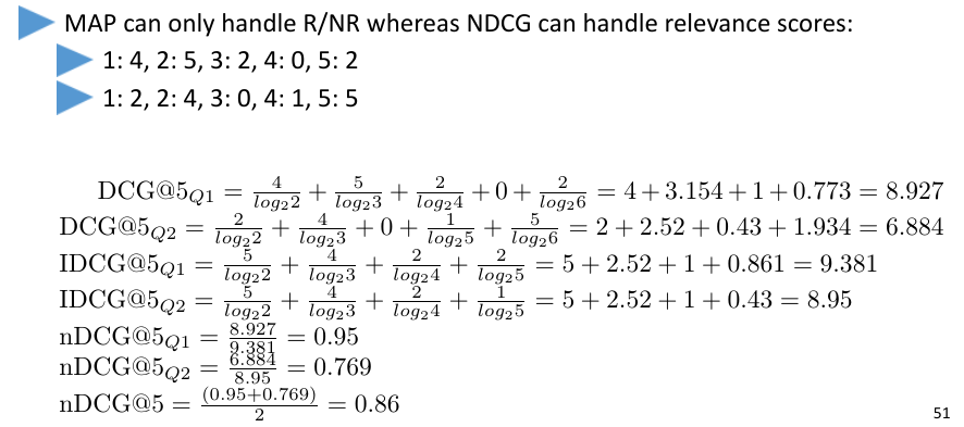
precision at K, MAP, NDCG, IDCG
15 elevance feedback and query expansion
17 text summarisation
18 question answering
Question 6: Vector space models, Word embeddings.
6 word embeddings
Word embeddings are word vectors that represent a word in terms of its context as projections of an original one-hot word vector into a lower dimensional space.
- why useful?
- allow representing words as dense vectors, where the dimensions reflect some notion of meaning. This facilitates the computation of semantic similarity between words.
- allows a relatively corpus independent representation of word meaning that is based on word distribution rather than pre-existing knowledge.
- rather than one-hot vectors allows meaningful dimensionality reduction in the feature space of text classifiers
onehot word vector
It is a vector representation of word, where the vector is the size of the vocabulary and the only value that is a one, is that corresponding to the index of the word. All other values in the vector are zero.
- results in sparse and high dimensional matrices.
- does not take into account word order or linguistic structure
vector space models,SVD
SVD: Frequent occurrence in similar contexts will indicate similarity.
- We build co-occurrence matrix (|V|x|V|) with offset ∆.
- We use SVD to decompose X as X=USV^T where:
- U(|V| x r) and V(|V| x r) are unitary matrices, and
- S(r x r) is a diagonal matrix.
- The columns of U (the left singular vectors) are then the word embeddings of the vocabulary.
- The word embeddings represent the projection of X into a lower dimensional space(also as higher demensional space)
Pros and Cons
- pros: perform well in a number of tasks
- pros:Uses global co-occurrence statistics efficiently as they operate on the entire corpus.
- cons
- Con: dimensions need to change as new words are added to the corpus, costly.
- Con: resulting vectors can still be high dimensional and sparse. only good at similarity, dimensions do not reflect meaning.
- Con: Quadratic cost to perform SVD.
Iteration based models
Word2vec
- Main intuition: Instead of computing co-occurrences from entire corpus, predict surrounding words in a window of length c of every word.
- Allows easier updates, faster to incorporate new words in model.
- Leads to low dimensional, dense vectors.
input and output of word2vec
input:
- a c x V matrix where each row is a one-hot vector representation of a word in a corpus, where the size of the vocabulary is assumed to be V. c is the size of the context window.
- the dimension N of the embeddings.
output
- the N x V embedding matrix projecting the one-hot vectors of the words to the embeddings space.
CBOW and skip-gram models
- Continuous bag of words model (CBOW): a language model where we have the context within a window sized c, predict a word.
- Skip gram model: having the word, predict its context.
PROS AND CONS: ITERATION BASED METHODS
- Pro: Do not need to operate on entire corpus which involves very sparse matrices.
- Pro: Can capture semantic properties of words as linear relationships between word vectors.
- Pro: Fast and can be easily updated with new sentences.
- Con: Can’t take into account the vast amount of repetition in the data.
Glove
- similar to word2vec:
- Count-based method instead of prediction-based.
- Does matrix factorisation for dimensionality reduction.
- Can leverage repetitions in the corpus as using the entire word co- occurrence matrix.
- train only on non-zero entries of co-occurrence matrix
- Computationally expensive for building matrix, then much faster as non-zero entries are not so many.
- Intuition: relationships between words should be explored in terms of their co- occurrence probabilities with some selected words k.
- evaluation
- extrinsic: test your model in a text classification, sentiment analysis..task does it outperform other methods? compare two models
- intrinsic: use datasets labelled with word similarities
16 recommender systems
collaborative filtering: based on users past behaviour, memory based
- user based: find similar users and recommend what they liked
- item based: find similar items to those I have previously liked
- PROS
- easy to implement, users and items can be treeated as IDs, no content need to be processed.
- preforms reasonably well when have a history of likes.
- cons
- cold start and pupularity bias
- cold start: There needs to be enough other users already in the system to find a match. New items need to get enough ratings.
- popularity bias: Hard to recommend items to someone with unique tastes. Tends to recommend popular items (items from the tail do not get so much data)
- can’t perform well when lack history
- context is ignored(restaurant in new city)
- cold start and pupularity bias
content-based
- features extracted from item contents
- ignore users preference
- PROS
- No need for data on other users. No cold-start problem.
- Able to recommend to users with unique tastes.
- Able to recommend new and unpopular items. No first-rater problem.
- We can provide better explanations of the reasons behind a recommendation, i.e. the features that the recommended item has in common with what they’ve viewed before.
- CONS
- Need to extract features from content, more difficult for e.g. video.
- Difficult to implement serendipity.
- Easy to overfit (e.g. for a user with few data points we may “pigeonhole” them).
new
5 spelling correction
Another dictionary word (real-word error). A non-dictionary word (non-word error).